Dysarthria is a speech disorder with symptoms similar to what is exhibited after a person has a stroke. In contrast to a stroke, this disorder can be present at birth and effect the individual throughout their life. There is a particularly high occurance rate of this disorder in China. When I was still in college, I was able to get my hands on a nicely curated data set consisting of mandarain speaking individuals. Given the opportunity, I figured it was a worth while cause to try to create a “pre-test” of sorts - something which those who do not have great access to health care could use to determine if they were afflicted - before seeking expensive medical expertise.

This post omits some of the nitty-gritty technical details. If interested, please reference the full research paper.

The Data

The data was collected by a physican in China, and consists of indivudals who are suffering from Dysarthia, as well as healthy speakers. I’m not entirely familiar with the language of Mandarin, but the participants were asked to speak, what roughly equates to English syllables, into a microphone. Both male and female individuals recorded the same syllables, and the physician labeled each participant as either “healthy” or “unhealthy.” There were 69 speakers in total, which is a small dataset by any measure. However, given the difficulty in creating such a medical dataset, this would prove to be a good launch point.

Pre-processing

The recorded syllables were in the form of WAV files. While there has been some interesting results stemming from feeding WAV files into the neural network directly, the files are oftentimes transformed before being fed to a neural network. In our case, we went with Mel-Frequency Cepstrum Coefficients (MFCCs). These are much smaller in size and generally capture the timbre of the audio.

The waveform $X$ is pre-processed into an MFCC feature vector $X′ = \{x_1, ..., x_t, ..., x_T \}$, where the number of MFCC frames $T$ can be different from one raw input $X$ to another. The MFCC vectors $x_t$ was created using a sliding window of 25 milliseconds with a 10 millisecond stride. Each MFCC vector consists of $N$ coefficients $x_t = \{θ_1, ..., θ_n, ..., θ_N \}$. We experimented with $N = \{13, 25, 29\}$.

Apart from the transfromation from raw WAV file to MFFC vectors, each MFCC coefficient was normalized such that the mean and variance for $θn$ was 0 across all training examples.

Because the value of $T$ can vary with the length of the WAV file, we padded each example in the mini-batch of 64 with values of 0, such that each MFCC vector $X'$ had the same length as the largest example in the batch, $T_max$.

The Model

Several models were used in our research. These include a one, as well as a two, layer one directional LSTM. We also experimented with a two layer bi-directional LSTM network. We feed pre-processed MFCC feature vector $X'$ into the LSTM in mini-batches of 64. We then cherry pick the output from the $T$th LSTM cell and send it to a linear regression layer, where a label $Y$ is produced.

To train, we used the Adam algorithm with a cross entropy loss. We did have some fun with early stopping to prevent overfitting. I’ll leave the details of that in the paper. We used 40 epochs as the maximum training length.

Ensuring 0-Value Padded MFCC vectors Are Not Processed

To prevent the 0 padding from affecting the predictions and training, we ensured that the model only used non-zero padding values while calculating their predictions.

Within the context of tensorflow, we can do this by supplying the dynamic_rnn constructor with a keyword parameter lengths. This takes the form of a list of integers which represent the length of each example in the batch. The length here refers the the number of non-zero padded MFCC vectors. To calculate the length, or number of non-zero padded $x_t$ values for each $X'$, we can use the following. Note that sequence is a tensor of size $[mini\_batch\_size, T_{max}, θ_N]$.

def getExampleLengths(self, sequence):
    used = tf.sign(tf.reduce_max(tf.abs(sequence), reduction_indices=2))
    lengths = tf.reduce_sum(used, reduction_indices=1)
    lengths = tf.cast(lengths, tf.int32)
    return lengths

In the code above, we first take the absolute value with respect to each MFCC in the example. Then, by using tf.sign(), we transform any values which are greater than 0 to a 1. We then sum up these “1” values, and we get the number of MFCC vectors which do not consist entirely of zeros. This is the number of non-padded MFCC vectors. The nuance we take advantage of here, is that the tf.sign() function returns 0 for values that are 0, as well as the fact that we take the absolute value first - ensuring MFCC vectors which unprobalistically add up to zero when summing up their nagative and positive values are not counted in the returned variable.

Cherry Picking the Final Weights

By virtue of the LSTM, each cell in an LSTM maintains its own weights. We are only interested in the weights of the final cell. That is, the layer which processes the final non-zero padded MFCC vector. To pluck out these weights from the whole LSTM network, we can use the code below.

def getLastOutput(self, output, exampleLengths):
    shape = tf.shape(output)
    batch_size = shape[0]
    max_length = shape[1]
    out_size = int(output.get_shape()[2])
    index = tf.range(0, batch_size) * max_length + (exampleLengths - 1)
    flat = tf.reshape(output, [-1, out_size])
    relevant = tf.gather(flat, index)
    return relevant

Here, output is a list of weights from each LSTM cell. We use a hidden layer size of 200, so output has the shape of $[mini\_batch\_size, T_{max}, 200]$. exampleLengths is the return value from the getExampleLengths() - a 1D vector of integers representing the amount of non-zero padded MFCC vectors in each example. We first calculate the shape of output. We must do this because the last batch could be smaller than 64 and $T_{max}$ varies by batch. We then create the variable index, which is a 1D tensor of integers which will be used to pluck out the relevant outputs - 1D tensors of shape [200] - after we completely flatten the output variable. We finally use tf.gather() supplied with the index variable to cherry-pick the outputs we want from a “flattened” 2D tensor flat of size $[(mini\_batch\_size * T_{max}), 200]$,

The Model Code

Other than the above, implementing the models is straight forward.

LSTM with One Layer

with tf.name_scope("lstm"):
    lstmCell = tf.contrib.rnn.LSTMCell(hidden_size)
    output, state = tf.nn.dynamic_rnn(lstmCell, X, sequence_length= lengths, dtype= tf.float32)
lastOutputs = self.getLastOutput(output, lengths)
return lastOutputs

LSTM with two Layers

You’ll notice we add dorpout in between the two layers of the LSTM below.

with tf.name_scope("lstm"):
  lstmCell = tf.contrib.rnn.LSTMBlockCell(hidden_size)
  dropoutlstmCell = tf.contrib.rnn.DropoutWrapper(lstmCell, input_keep_prob= 0.5,
						  output_keep_prob= 0.5)
  stackedLstmCell = tf.contrib.rnn.MultiRNNCell([lstmCell, dropoutlstmCell])
  output, state = tf.nn.dynamic_rnn(stackedLstmCell, X,
				    sequence_length= lengths,
				    dtype= tf.float32)
lastOutputs = self.getLastOutput(output, lengths)
return lastOutputs

Two Layer Bi-Directional LSTM

You can see that we grab the final weights from both passes. We end up concatenating these and passing them to the linear regression layer.

lengths = self.getExampleLengths(X)
with tf.name_scope("lstm"):
  lstmCell = tf.contrib.rnn.LSTMBlockCell(hidden_size)
  output, _ = tf.nn.bidirectional_dynamic_rnn(lstmCell, lstmCell, X,
						  sequence_length= lengths,
						  dtype= tf.float32)
lastForwardOutputs = self.getLastOutput(output[0], lengths)
lastBackwardOutputs = self.getLastOutput(output[1], lengths)
lastOutputs = tf.concat([lastForwardOutputs, lastBackwardOutputs], axis= 1)

return lastOutputs

Results

We conducted several experiments in the paper. For this post, I’ll include the first experiment, and one other - which eachieved the most fruitful results.

Comparison to a Baseline

We first wanted to compare the LSTM against a baseline on a relatively easy task, which we call “Known Speakers.” We shuffle up the syllables from all speakers and partition them into a training, validation, and testing set with a 2:1:1 ratio. Some syllables from the same speaker can easily end up in more than one partition. We then evaluated the accuracy at a syllable level for a baseline, 1-layer fully connected neural network, and our three LSTM models.

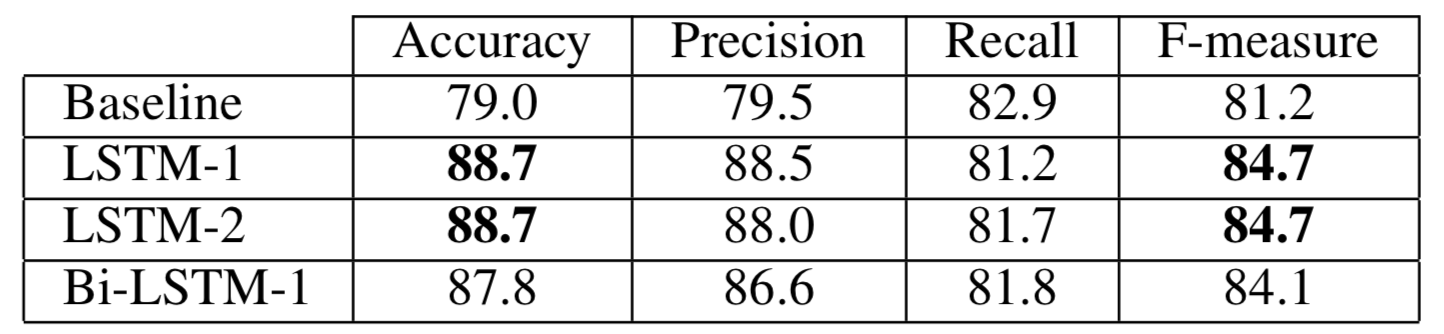
A majority classifier would achieve 53% accuracy on this dataset. The baseline is a large improvement, but the LSTM networks come out on top.

Best Results

The following illustrates the experiment with the most fruitful results. Several methodologies differ between the baseline experiment and this one, so first these are explained.

Patient Level Evaluation

The first experiment was fun, but int he real world, we don’t care much about classifying each syllable as either “healthy” or “unhealthy.” We want to diagnose patients by taking into account any relevant information. Meaning, we need to somehow transform a set of syllable predictions, and aggregate them into one prediction for the patient. We employed two different methods: soft-majority, and a normalized nosiy-OR. They ended up producing absolutely identical results. The equations are below. We calculated the nosiy-OR in log-space and normalized by the number of syllables $m$ because each speaker can have a varying number of syllables. This allowed us to directly compare the scores across speakers with such a variance in the number of training examples they provided.

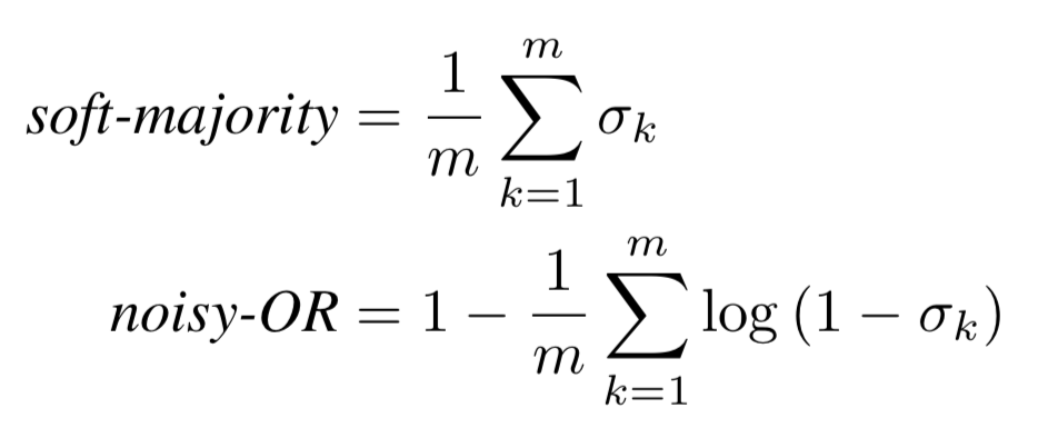
Where $σ_k$ is prediction from the linear regression layer for a specific syllable.

Novel Speakers

We need to ensure that the models work on speakers which have never been presented to the model before. To achieve this, we used k-fold validation to evaluate the performance of our models. The speakers were shuffled, 9 of them were peeled off for a validation group, and the other 60 were split into 10 folds. We performed 10 training runs, for a max of 40 epochs, where 9 folds were used for training and the last fold was used for testing. We through away the weights after each run.

Specific Syllables / Vowels

We found that certain syllables exhibit dysarthria much more so than others. In this experiment, we determine the effects of considering only a subset of the syllables. There are two particular groups of syllables, or vowels, that we experimented with removing from the training, testing, and validation sets. These include compound vowels cv and consonants with consanant /a/. We simply followed the k-fold validation process discussed, but omitted these vowels in the full dataset, before partitioning into the validation, training, and testing sets.

The Final Outcome

We report the ROC score generated by fluctuating the threshold which dictates whether the number derived from the soft-majority method should be interpreted as a “healthy” or “unhealthy” diagnoses. The numbers are below.

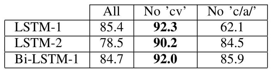
As you can see, the LSTM-1 model, which is a uni-directional, one-layer LSTM, takes the crown with 92.3 AUC score. Not bad at all considering the small dataset, and the fact that the hidden size was a mere 200 weights!

Conclusion

Hopefully this will be of use to anyone interested in the medical side of Machine Learning or someone looking for practical LSTM examples in Tensorflow. Unfortunately I cannot publish the full repo, as the pipeline includes medical data and I have no intention of violating HIPPA. Please reach out via the links in the sidebar or my email below if you have specific questions!

The paper also includes experiments relating to the number of cepstrums included, which did end up getting the Bi-LSTM-1 to a 90.4 AUC score with 25 cepstrums included. To see all the graphs, math, and methodology - check out the paper!